I am pretty new when it comes to the Husky and NewAE products as a whole. I went through the first few starter Juypter notebook labs(Three recommended by Lab 0) with no issue and decided to do SCA101 Lab 2 1A with the SAM4S.
My issue is I cant tell a difference between the traces when I modify the simple serial function. I have run through the lab about 3 or 4 times now to check if I am doing something wrong.
I added some info for one of the times I did the lab so hopefully someone can help me sanity check myself. Is the SAM4S just hard to tell the difference or did I do something wrong?
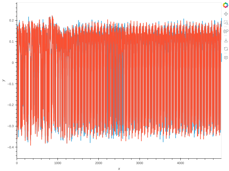
Also I am a new user so I am only allowed to attach one embedded media. I picked to include the graph that overlays the multiplication and division I did at the end. I assumed these would show some obvious active or idle states of the target.
Lab Info
SCOPETYPE = 'OPENADC'
PLATFORM = 'CWHUSKY'
cd ../../../firmware/mcu
mkdir -p simpleserial-base-lab2 && cp -r simpleserial-base/* $_
cd simpleserial-base-lab2
%%bash -s "$PLATFORM"
cd ../../../firmware/mcu/simpleserial-base-lab2
make PLATFORM=$1 CRYPTO_TARGET=NONE
Connect to husky using provided code - Output
INFO: Found ChipWhisperer😍
scope.gain.mode                          changed from low                       to high
scope.gain.gain                          changed from 0                         to 22
scope.gain.db                            changed from 15.0                      to 25.091743119266056
scope.adc.samples                        changed from 131124                    to 5000
scope.clock.clkgen_freq                  changed from 0                         to 7363636.363636363
scope.clock.adc_freq                     changed from 0                         to 29454545.454545453
scope.clock.adc_rate                     changed from 0.0                       to 29454545.454545453
scope.io.tio1                            changed from serial_tx                 to serial_rx
scope.io.tio2                            changed from serial_rx                 to serial_tx
scope.io.hs2                             changed from None                      to clkgen
scope.io.cdc_settings                    changed from [1, 0, 0, 0]              to [0, 0, 0, 0]
scope.glitch.phase_shift_steps           changed from 0                         to 4592
scope.trace.capture.trigger_source       changed from trace trigger, rule #0    to firmware trigger
cw.program_target(scope, prog, "../../../firmware/mcu/simpleserial-base-lab2/simpleserial-base-{}.hex".format(PLATFORM))
def capture_trace(_ignored=None):
    ktp = cw.ktp.Basic()
    key, text = ktp.next()
    return cw.capture_trace(scope, target, text).wave
wave = capture_trace()
print("✔️ OK to continue!")
wave = capture_trace()
cw.plot(wave)
output:
(Replace simple serial code with volatile variable multiplication)
Recompile and upload
wave2 = capture_trace()
cw.plot(wave2)
output:
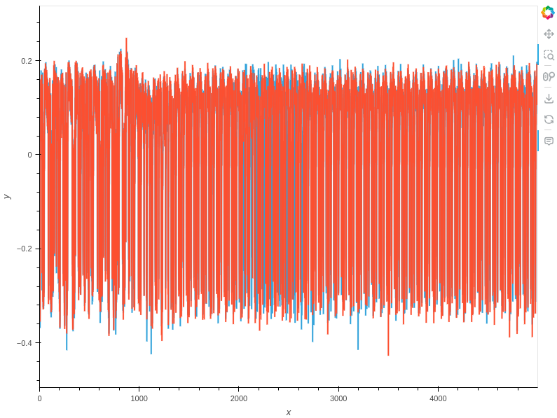
cw.plot(wave) * cw.plot(wave2)
output:
(Replace simple serial code with for loop that multiples a volatile variable 1000 times.
Recompile and upload
wave3 = capture_trace()
cw.plot(wave3)
(Swap out multiply for divide in the simple serial for loop)
Recompile and upload
wave4 = capture_trace()
cw.plot(wave4) * cw.plot(wave3)
output: